
SESTransient
SESTransient, the successor of AutoTransient, automates the analysis of transient phenomena with the FFTSES and HIFREQ engineering modules.
Similar to its predecessor, SESTransient runs FFTSES and HIFREQ in turn, using computation frequencies recommended by FFTSES to run HIFREQ, until user-defined termination criteria are met. However, with this integrated and streamlined version of AutoTransient, SESTransient is more integrated, advanced and powerful.
Technical Highlights
SESTransient includes every capability of AutoTransient, and much more:
- FFTSES and HIFREQ template files are designed within one streamlined interface.
- Flexibility to import existing template HIFREQ & FFTSES files, or to design a network system with SESCAD.
-
Interactive conductors selection through the Network 3D Viewer:
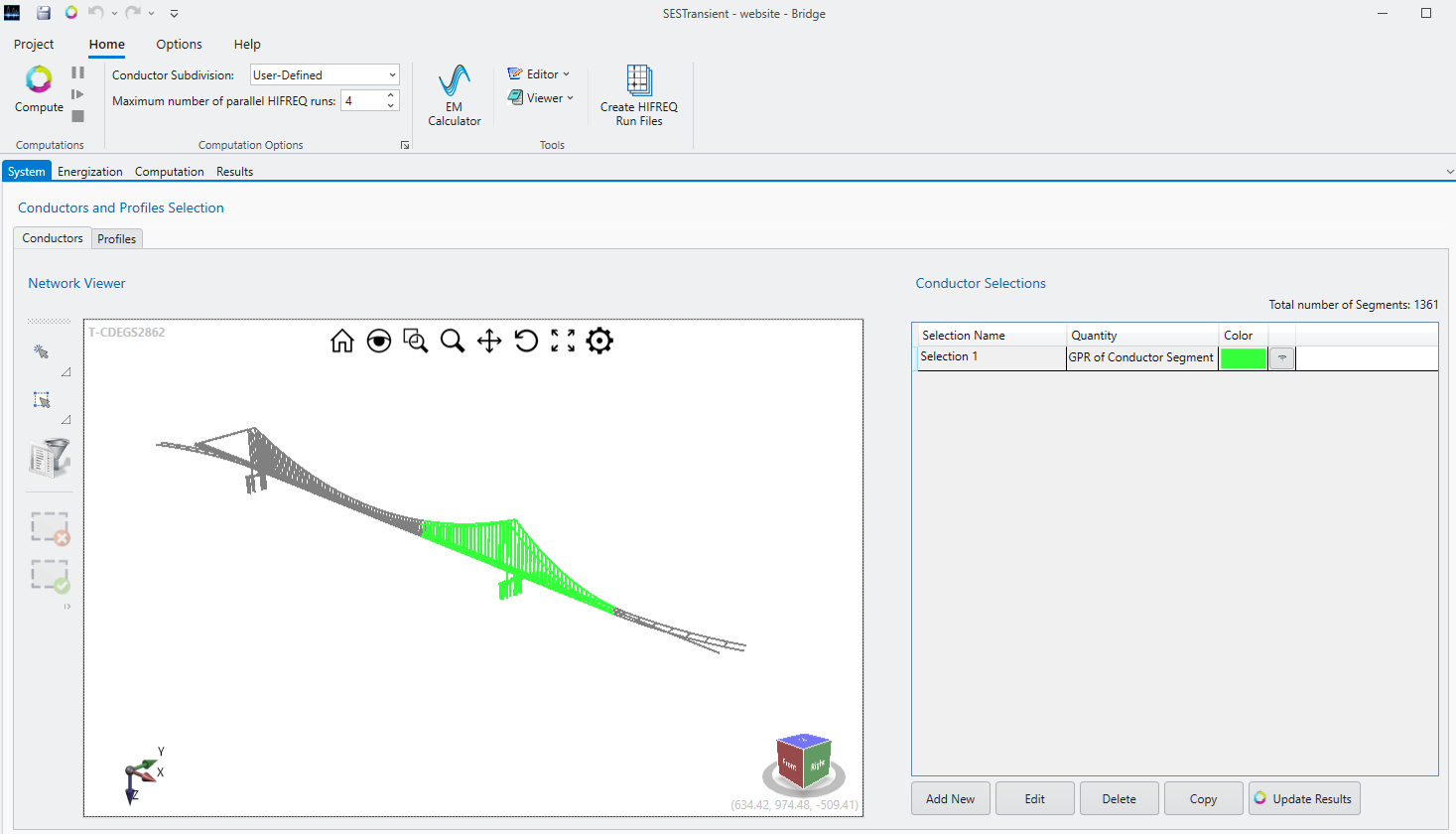
- Further refinement of conductor selection(s) can be done by filtering according to criteria such as: Depth, Radius, Coating Type, Conductor Type, Length, Segment Number, Conductor Number or Cable Type.
-
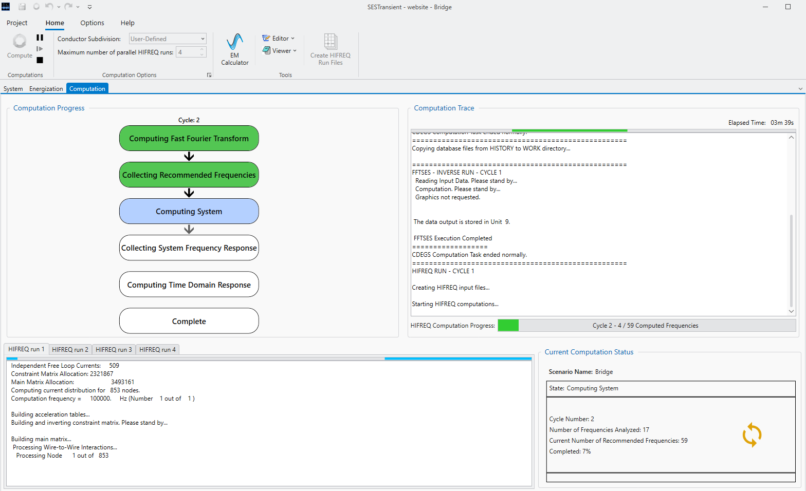
Users with multiple-core processors can run multiple HIFREQ computations in parallel, making the iterative process of running the HIFREQ module much more efficient and less time‑consuming:
-
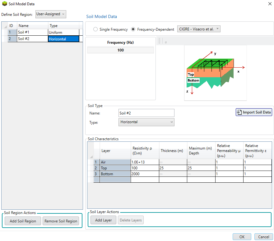
Integration of frequency dependent soil models. The electrical characteristics of soil varies with frequency, and SESTransient enables the specification of soil models that are frequency dependent. There are two options:
Results can also be exported in a CSV file format for further examination of computed values.
![]()
![]()
![]()
[1] S. Visacro, Rafael Alipio, “Frequency Dependence of Soil Parameters. Effect on the Lightning Response of Grounding Electrodes”, IEEE Transactions on Electromagnetic Compatibility, vol. 55, 2013.